Loading a Pretrained TOP Model and Performing Chemical Ordering Optimization

This tutorial demonstrates how to load a pretrained TOP model and perform a chemical ordering optimization using the npl library.

First, we need to import the necessary modules and initialize the TOPCalculator with the ExtendedTopologicalFeaturesClassifier.

from npl.descriptors import ExtendedTopologicalFeaturesClassifier
from npl.calculators import TOPCalculator

calc = TOPCalculator('ETOP', stoichiometry='Pt151Cu50',
                     feature_classifier=ExtendedTopologicalFeaturesClassifier)

etop = calc.get_feature_classifier()

When the TOPCalculator is initialized, it will load the topological parameters for the given stoichiometry. You should see output similar to the following:

INFO - Loading top parameters of Pt151Cu50
INFO - Parameters obtained from reference: L. Vega Mater. Adv., 2021, 2, 6589-6602
INFO - Parameters loaded successfully
INFO - Parameters:
{'CuPt': -25.0, 'Cu(cn=6)': 267.0, 'Cu(cn=7)': 342.0, 'Cu(cn=8)': 372.0, 'Cu(cn=9)': 372.0}

Next, we will run 20 Monte Carlo simulations to optimize the chemical ordering.

from npl.monte_carlo import run_monte_carlo
from npl.core import Nanoparticle

beta = 250
max_steps = 10000

energy_calculator = calc
feature_classifier = etop

energies_MC, steps_MC = [], []
for i in range(10):
    start_particle = Nanoparticle()
    start_particle.truncated_octahedron(7, 2, {'Pt': 151, 'Cu': 50})
    best_particle, accepted_energies = run_monte_carlo(beta, max_steps,
                                                       start_particle,
                                                       energy_calculator,
                                                       feature_classifier)
    min_energy, min_step = min(accepted_energies, key=lambda x: x[0])
    energies_MC.append(min_energy)
    steps_MC.append(min_step)
    if min_energy <= min(energies_MC):
        global_minimum = best_particle

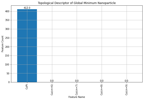
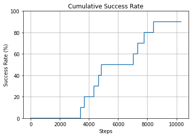
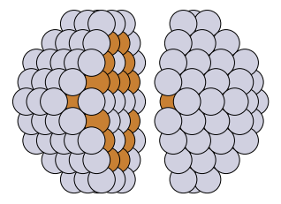
Finally, we evaluate the results of our Monte Carlo simulations by looking at the cumulative success rate plot and visualizing the global minimum chemical ordering. We also plot its resulting topological descriptor.

from npl.visualize import plot_cummulative_success_rate

plot_cummulative_success_rate(energies_MC, steps_MC)

from npl.visualize import plot_parted_particle

plot_parted_particle(best_particle)

threshold = 1e-16
filtered_indices = [i for i, coef in enumerate(calc.coefficients) if abs(coef) > threshold]
feature_names = feature_classifier.get_feature_labels()

feature_vector = best_particle.get_feature_vector(feature_classifier.get_feature_key())
filtered_feature_vector = [feature_vector[i] for i in filtered_indices]
filtered_feature_names = [feature_names[i] for i in filtered_indices]

# Plot the filtered feature vector
plt.figure(figsize=(10, 6))
bars = plt.bar(filtered_feature_names, filtered_feature_vector)
plt.xlabel('Feature Name')
plt.ylabel('Feature Count')
plt.title('Topological Descriptor of Global Minimum Nanoparticle')
plt.xticks(rotation=90)
plt.grid(True)

# Annotate bars with their heights
for bar in bars:
    yval = bar.get_height()
    plt.text(bar.get_x() + bar.get_width()/2, yval, round(yval, 2), ha='center', va='bottom')

plt.show()