Training a Topological Surrogate Energy Model

In this document, we will walk through the steps to train a surrogate energy model for nanoparticles using Topological Descriptors. Here, we import essential modules that will allow us to create nanoparticles, compute their energies, extract features, and perform Bayesian Ridge Regression.

from npl.core import Nanoparticle
from npl.calculators import EMTCalculator
from npl.descriptors.global_feature_classifier import testTopologicalFeatureClassifier
from npl.calculators import BayesianRRCalculator
from npl.utils.utils import plot_learning_curves
import numpy as np
import matplotlib.pyplot as plt
import pickle

This function initializes an EMTCalculator and creates a list of nanoparticles based on the given parameters. Each nanoparticle’s energy is computed and stored in the training set.

def create_octahedron_training_set(n_particles, height, trunc, stoichiometry):
    emt_calculator = EMTCalculator(fmax=0.2, steps=1000)

    training_set = []
    for i in range(n_particles):
        # Initialize a new Nanoparticle instance
        p = Nanoparticle()
        # Create a truncated octahedron nanoparticle with specified parameters
        p.truncated_octahedron(height, trunc, stoichiometry)
        # Compute the energy of the nanoparticle using the EMT calculator
        emt_calculator.compute_energy(p)
        # Add the nanoparticle to the training set
        training_set.append(p)

    return training_set

Here, we define the stoichiometry for our nanoparticles and generate a training set containing 40 nanoparticles.

stoichiometry = {'Pt': 55, 'Au': 24}
training_set = create_octahedron_training_set(40, 5, 1, stoichiometry)

We initialize the TopologicalFeatureClassifier to compute the topological features for each nanoparticle in the training set.

classifier = testTopologicalFeatureClassifier(list(stoichiometry.keys()))
for p in training_set:
    classifier.compute_feature_vector(p)

An instance of the Bayesian Ridge Regression calculator is created, and we fit the model using the training set with 10% of the data reserved for validation.

calculator = BayesianRRCalculator(classifier.get_feature_key())
calculator.fit(training_set, 'EMT', validation_set=0.1)

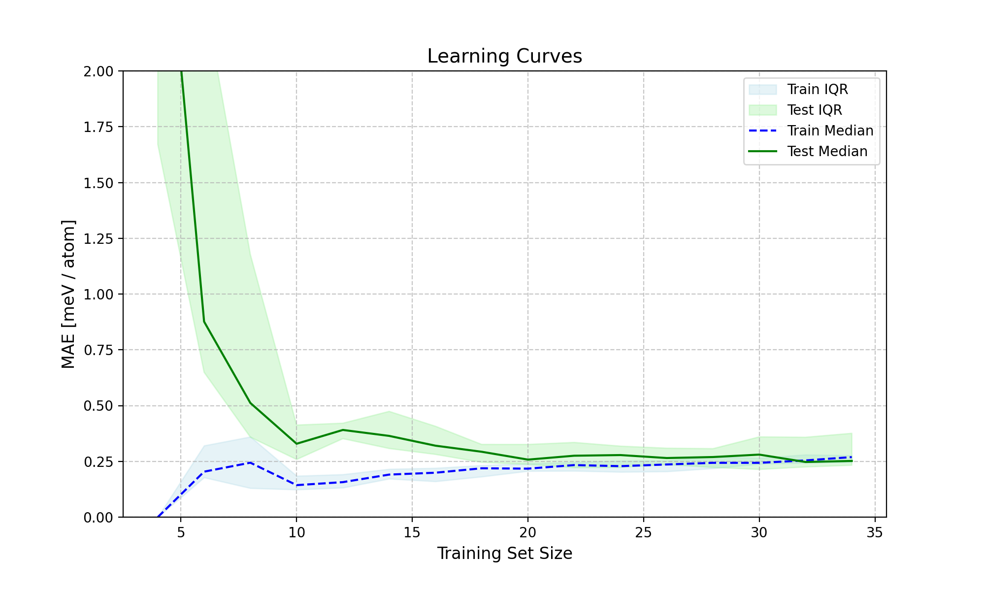
This figure illustrates the learning curve for the model, depicting the training and test performance as the training set size increases.

X = [p.get_feature_vector('TFC') for p in training_set]
y = [p.get_energy('EMT') for p in training_set]
n_atoms = training_set[0].get_n_atoms()
plot_learning_curves(X, y, n_atoms, calculator.ridge, n_splits=10, train_sizes=range(4, 30, 2), y_lim=(0, 2))

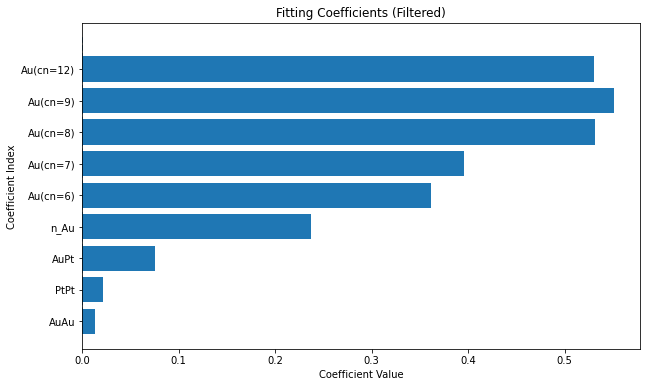
We plot the coefficients values to visualize the importance of each feature in the model.

coefficients = calculator.get_coefficients()
feature_names = classifier.get_feature_labels()
plt.figure(figsize=(10, 6))
plt.bar(range(len(coefficients)), coefficients)
plt.hlines(0, 0, len(coefficients), linestyles='dashed')
plt.xticks(range(len(coefficients)), feature_names, rotation=90)
plt.xlabel('Coefficient Index')
plt.ylabel('Coefficient Value')
plt.title('Fitting Coefficients')
plt.show()

Finally, we save the trained model to a file for future use, ensuring that we can reuse it without retraining.

calculator.save('bayesian_rr_calculator.pkl')