Chemical Ordering Global Optimization

In this tutorial, we demonstrate the global optimization of chemical ordering in nanoparticles using Monte Carlo and basin-hopping algorithms.

from npl.core import Nanoparticle
from npl.descriptors.local_environment_feature_classifier import LocalEnvironmentFeatureClassifier
from npl.calculators import BayesianRRCalculator
from npl.descriptors.global_feature_classifier import testTopologicalFeatureClassifier
from npl.utils.utils import plot_cummulative_success_rate
import numpy as np
import matplotlib.pyplot as plt
from ase.visualize import view

Creating the Nanoparticle and Optimizing

Define a function to initialize a random particle:

def create_start_particle(height, trunc, stoichiometry):
    start_particle = Nanoparticle()
    start_particle.truncated_octahedron(height, trunc, stoichiometry)
    return start_particle

This function generates a nanoparticle with a specific stoichiometry.

Loading the Bayesian Ridge Regression Model

Load a pre-trained Bayesian Ridge Regression model and extract coefficients:

global_energy_calculator = BayesianRRCalculator.load('bayesian_rr_calculator.pkl')
global_topological_coefficients = global_energy_calculator.get_coefficients()
print(global_topological_coefficients)

Compute coefficients and set up the model for local calculations:

from npl.calculators.energy_calculator import compute_coefficients_for_linear_topological_model
coefficients, total_energies = compute_coefficients_for_linear_topological_model(
    global_topological_coefficients, symbols, n_atoms)

Running Monte Carlo Simulation

Perform Monte Carlo simulation with the energy calculator:

from npl.monte_carlo import run_monte_carlo as rmc

steps_MC, energies_MC = [], []
for i in range(10):
    start_particle = create_start_particle(4, 1, {'Au': 0.33, 'Pt': 0.67})
    beta, max_steps = 250, 10000
    [best_particle, accepted_energies] = rmc(beta, max_steps, start_particle, energy_calculator, local_feature_classifier)

    min_energy, min_step = min(accepted_energies, key=lambda x: x[0])
    energies_MC.append(min_energy)
    steps_MC.append(min_step)
    if min_energy <= min(energies_MC):
        global_minimum = best_particle

Visualizing Results

Use ASE to view the optimized particle and plot accepted energies:

plot_atoms(global_minimum.get_ase_atoms(), rotation=('0x,+180y,0z'))
plt.axis('off')

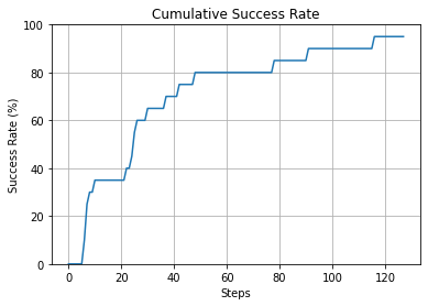
Plot the cumulative success rate:

plot_cummulative_success_rate(energies_MC, steps_MC)

Running the Optimizal Exchange Algorithm

Run the optimal exchange algorithm to search for global minima:

from npl.optimization.basin_hopping import run_basin_hopping
steps_BH, energies_BH = [], []
for i in range(20):
    start_particle = create_start_particle(4, 1, {'Au': 0.33, 'Pt': 0.67})
    [best_particle, lowest_energies, flip_energy_list] = run_basin_hopping(
        start_particle, energy_calculator, total_energies, 100, 5)
    energies_BH.append(lowest_energies[-2][0])
    steps_BH.append(lowest_energies[-2][1])

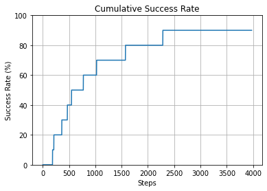
Plot the cumulative success for the Optimal Exchange algorithm: